Epilog
Beta and Bit returned to their times only because they discovered the rules governing the time vehicle. The noticed in what way the year into which they travelled depended on the number entered into the driver of the time machine and used that information in practice. Ability to notice such relationships may come in handy not only during intrusion into study of a crazy mathematician. The world that surround us is bristling with many relationships. We may use a skill of noticing and employing them in various situations.
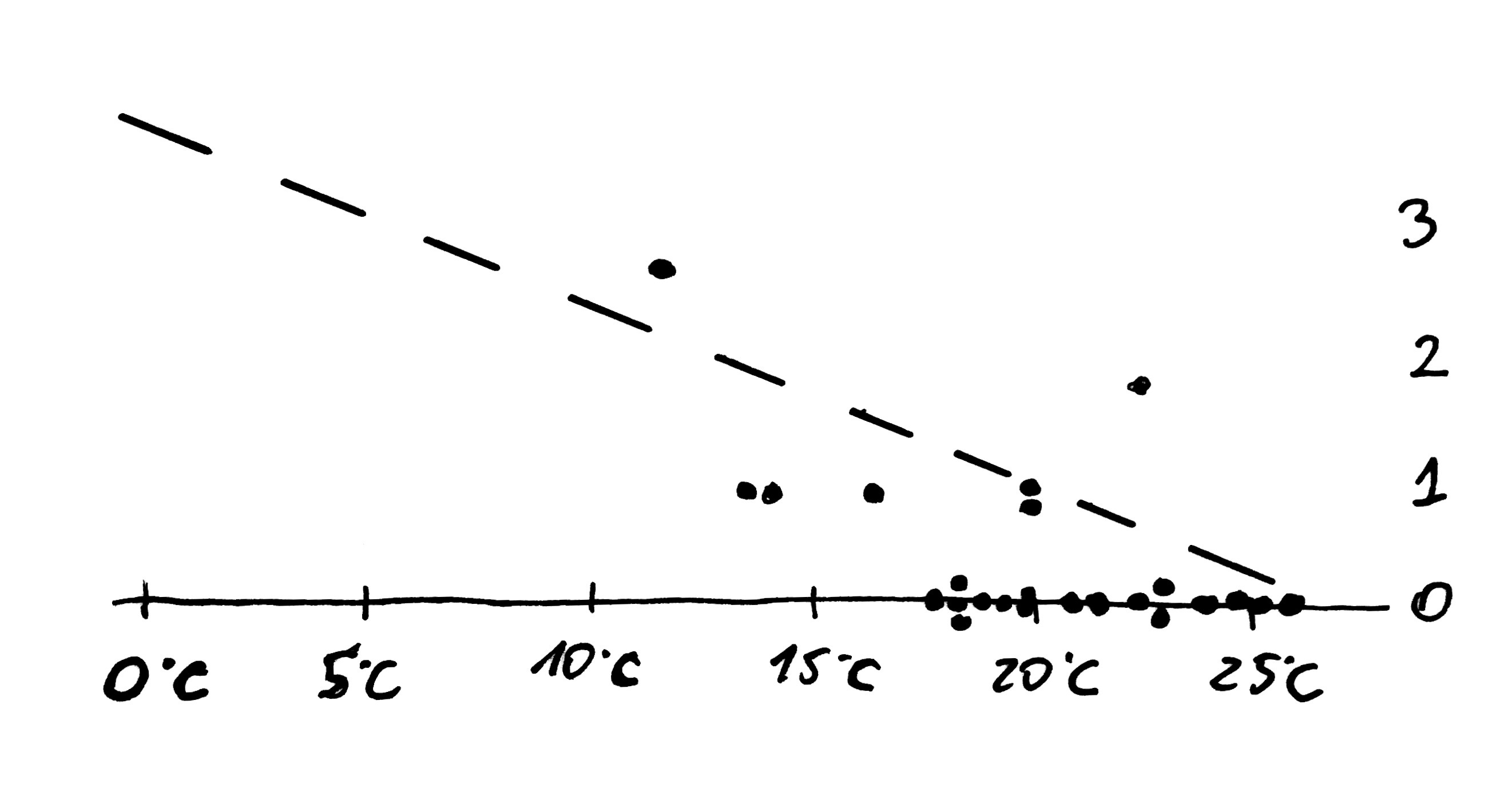
This skill allowed the scientists to explain the Space Shuttle Challenger disaster which occurred in 1986. 45 seconds after the launch of the rocker the spectators could see a flame of fire which quickly led to disintegration of the whole shuttle. The disaster claimed the lives of the whole crew. It raised questions about the future of NASA. A special commission, which was established with a view of explaining the cause of the disaster, looked for any clues for a long time. Richard Feynman, physicist and later Nobel Prize winner, was a member of the commission. He noticed that low temperature decreases elasticity of O-rings sealing the rocket booster. Low elasticity translated into higher failure frequency. Even at temperature below 18C problems with O-rings occurred and the lower the temperature, the frequency of problems rocketed. The elasticity of the rubber rings was too small at 10C while during the night prior to the shuttle launch the temperature fell below 0C.
The following dot chart presents the results of the initial measurement of the number of temperature-related damage. All measurements were collected at temperature between 10 and 25C. It is obvious that the lower the temperature, the higher rate of damage. Had the scientist known that relationship, would they have been able to predict such a serious damage at 0C?
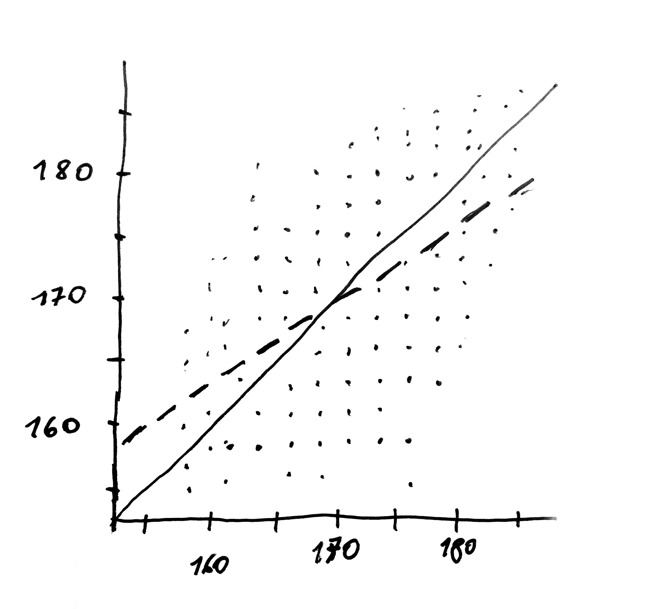
Regression is a method for identifying relationships between variables. Where does its name come from? Actually, the story behind it is very interesting. In 1886 sir Francis Galton was studying relationship between height of adult sons and height of their parents. He observed that sons of tall parents were usually tall but not as tall as the parents. Obviously, some sons were exceptionally tall and outgrew their parents. Yet when he examined the averages, he found out that the average height of children was somewhere in between the height of the parents and the average height of all children. Galton called that tendency ‘regression toward mediocrity’.
The following diagram illustrates Galton’s results. He examined over 1000 families. Dots located at OX axis display the weighted average height of parents while dots at OY axis present the height of children. The solid line represents the relationship corresponding to equal height of parents and children. The dashed line is the relationship reflected by the data. The average height of children is closer to the horizontal line. In contrast to the pairs of numbers collected by Beta and Bit, the measurement points are not placed ideally along the line. The line describing the relationship determined with that method is a line located as closely as possible to all the points.
Someone might ask about the value of such studies. What can we gain from the knowledge that average height of children is partially determined by the height of parents and partially it is not? Yet it turns out that the technique of linear regression paved the way for a huge progress in agriculture and cow breeding. When we know what part of cow’s milkiness is a genetic heritage coming from the bull and what part comes from the cow, we can use that knowledge to assess the breeding value of an animal. Nowadays the assessments of the breeding value are conducted on a large scale. They frequently include a complex pedigree of animals. Such assessments helped to increase milkiness of cows – it is estimated that in developed countries milkiness was tripled over the last 50 years! Such studies are based on nothing else but regression.
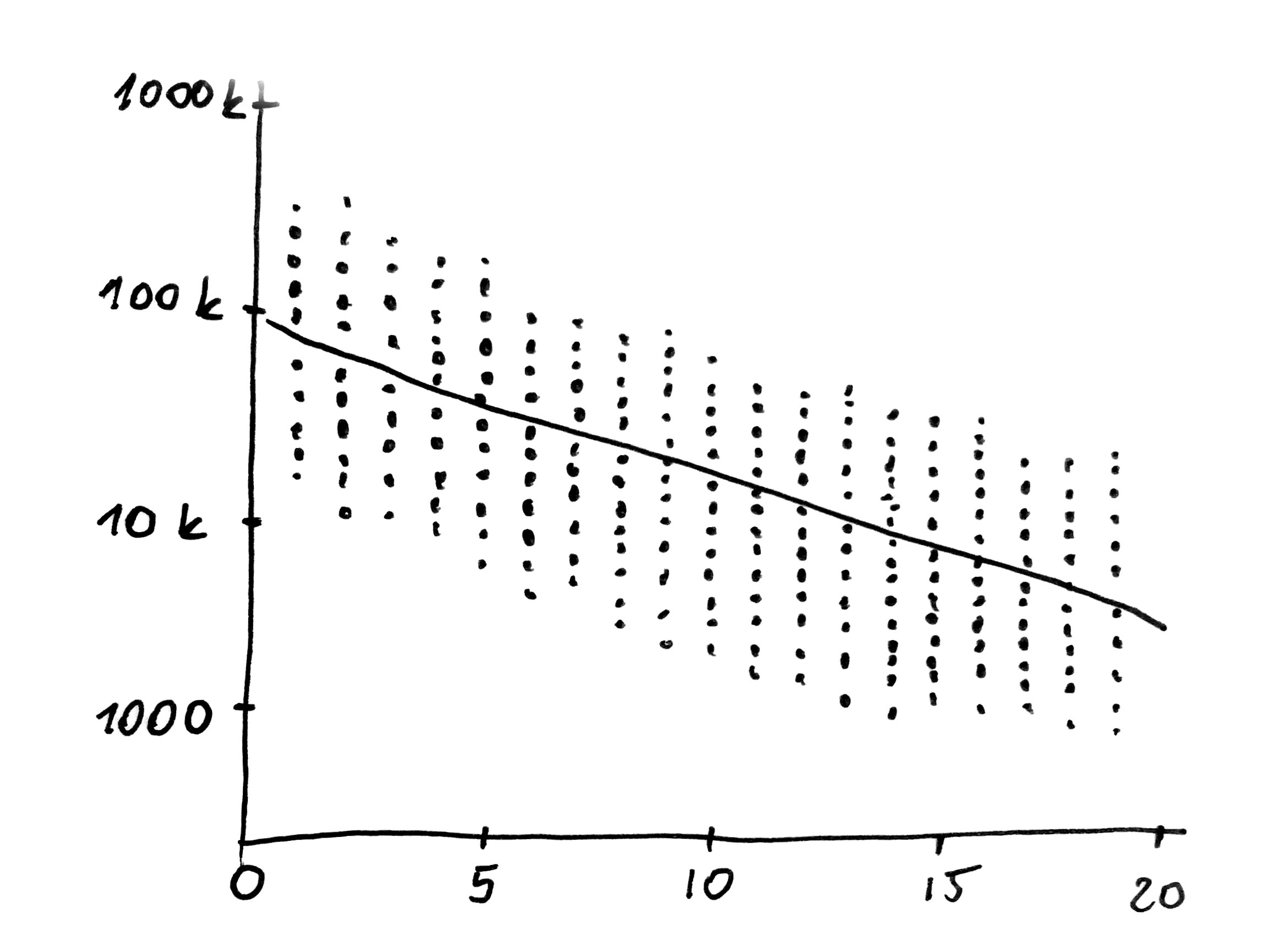
Now you will probably ask what is the use of regression in every-day life? Well, it is very useful and this fact can be easily proven. Let’s assume that we want to buy or sell a second-hand car or a flat or a mobile phone. We are wondering what may be the cost of a 5-year-old Volkswagen Passat with average equipment. Portals offering second-hand cars will display hundreds of sale offers. We can download that data and search for a relationship between a car’s age and its price. What would we discover? If we plot price logarithm against the cars’ age, a beautiful linear relationship will appear to our eyes. Where does this logarithm come from? It turns out that value of the cars drops with every year by a fixed percentage, which is around 15% (the exact value depends on the make and equipment). After a year a car’s price falls by 15%, after two years it falls by 27,8% (how come such percentage? here compound interest comes in handy), after three years by 38,6% and so on. However, when we take the logarithm of both sides of the price, compound interest changes into a linear relationship allowing us to quickly estimate the prices of second-hand cars.
The following diagram presents the relation between price expressed in exponential scale displayed on OY axis and car’s year of manufacture displayed on OX axis. The data was downloaded from otomoto.pl portal.
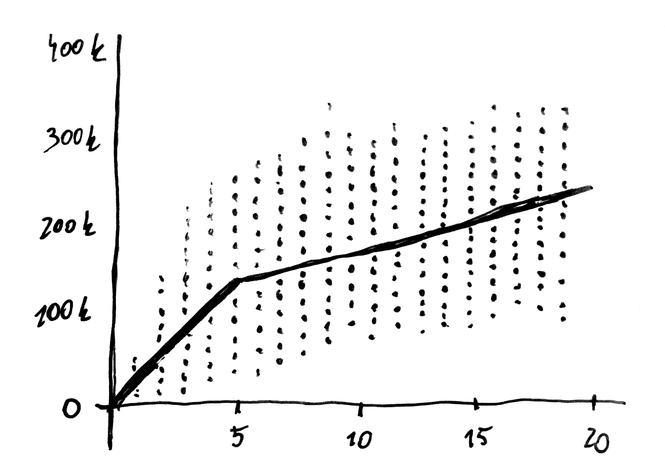
However, not every relationship is linear. Continuing the subject of second-hand cars, let us look at a very interesting relation between mileage and year of manufacture.
We would expect that mileage should increase in proportion to age of cars. If a certain number of kilometers was covered in a given year, then during two years the double number of kilometers should be covered, right? Interestingly, when we examine a chart presenting relation between mileage and age of cars, we observe a different trend for cars under 5 and a different trend for older vehicles. Young cars increase their mileage with rate of 20-25 thousand kilometers a year but after 5 years their mileage starts to increase by only 10-15 thousand kilometers a year. This dependence may result from difference in behavior of owners of older cars (sales representatives cover the highest number of kilometers and it is this group which most often drives new cars which are later on sold to new owners) or difference in behavior of sellers (they reduce mileage of the cars with high mileage and in case of older cars no service booklet is kept which would stand as a proof of manipulation).
We need to be careful when we search for relationships between variables. The fact that two variables seem dependent does not necessarily mean that one is a cause of the other. For example, when we analyze data about birth rate and number of stork nests in different villages in Poland, it turns out that there is a very strong dependence between these two values. The more nests, the more children! However, this does not prove that storks bring babies. So what does this prove? The bigger the village, the more houses, roofs, poles and other place for nests it has. On the other hand, more houses and people mean more children, obviously. This is why the number of children and the number of storks are related – they depend on the number of habitations.